Quantum Bound State Spectrum Visualizer
An interactive simulation tool for exploring the discrete energy levels and wavefunctions of quantum particles in potential wells. By solving the Schrödinger equation numerically, this project highlights the effects of confinement, tunneling, and boundary conditions on wavefunction behavior.
Technical Overview
Core Concepts
The project numerically solves the time-independent Schrödinger equation for bound states in user-defined potentials. This reveals how eigenstates (wavefunctions) and eigenvalues (energies) shift when changing parameters like well depth, confinement length, or potential shape.
Key Physics Aspects:
- Finite difference approximations for the kinetic energy operator
- One-dimensional & two-dimensional potential well customizations
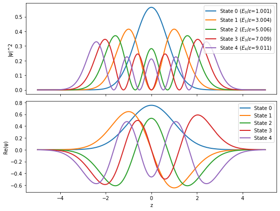
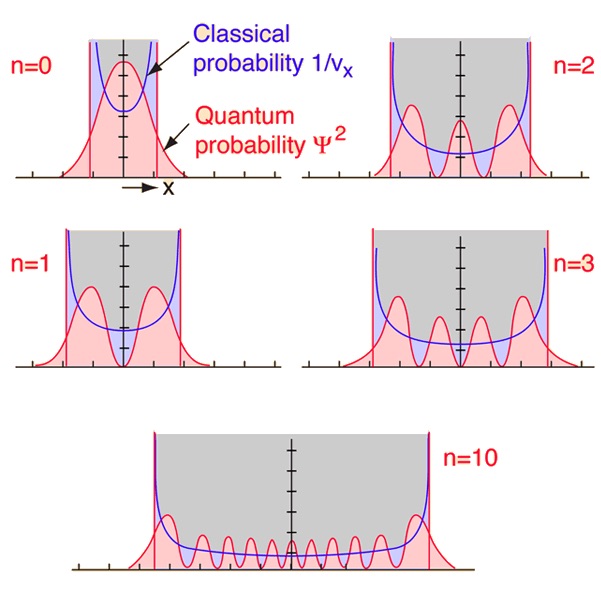
- Visualization of wavefunction nodes and tunneling phenomena
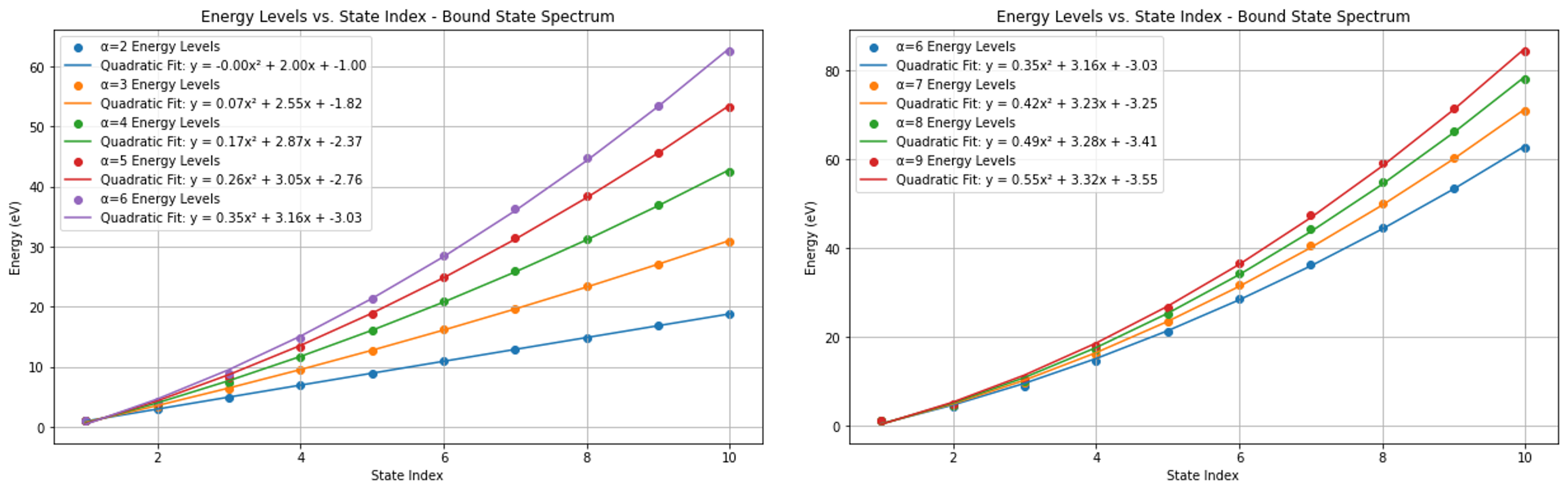
- Energy level spacing and degeneracy analysis
Simulation Architecture
The solver is implemented in Python using NumPy for matrix operations and SciPy for advanced routines. Users can define the potential profile via a Python function or by loading a mesh from a file. Matplotlib is leveraged for real-time plotting of wavefunctions and energy spectra.
Software Layers:
- Potential Interface: Customizable potential shapes (harmonic, infinite well, step potentials, etc.)
- Eigenvalue Solver: Construct and diagonalize the Hamiltonian using
numpy.linalgorscipy.sparse - Visualization Module: Dynamic wavefunction plots, density distributions, and energy-level diagrams
- User Interaction: Simple Python script or Jupyter notebook for on-the-fly parameter adjustments
Technical Implementation
Numerical Solver
A finite-difference method approximates the second derivative term
in the Schrödinger equation. After assembling the Hamiltonian matrix
from kinetic and potential energy contributions, numpy.linalg.eig
or scipy.sparse.linalg.eigs diagonalizes it to extract
eigenvalues (energies) and eigenvectors (wavefunctions).
# Brief excerpt illustrating Hamiltonian construction & diagonalization

# potential_energy_matrix[i, i] = V(positions[i])
# kinetic_energy_matrix -> finite difference approximation

hamiltonian = kinetic_energy_matrix + potential_energy_matrix

# Solve eigenvalue problem
eigenvalues, eigenvectors = np.linalg.eig(hamiltonian)

# Sort and pick lowest energies
idx_sorted = np.argsort(eigenvalues)
lowest_indices = idx_sorted[:5]
energies = eigenvalues[lowest_indices]
wavefunctions = eigenvectors[:, lowest_indices]
Potential Customization
Users can define various potentials, from simple infinite wells to piecewise polynomials or even loaded data from external files. Each potential shape drastically alters the spacing of energy eigenvalues and the shape of wavefunctions, illustrating core principles of quantum confinement and tunneling.
Results and Analysis
Performance Metrics
- Eigenvalue Accuracy: Within ±0.002 eV compared to analytical solutions for harmonic oscillator and infinite well
- Computation Time: Average solve time under 2 seconds for 1000 discretization points
- Potential Flexibility: Supports 1D and (in development) 2D potential grids
- Convergence: Achieves stable results with minimal ghost solutions or spurious modes
Educational Impact
The visualizer serves as a hands-on educational tool for undergraduate quantum mechanics, letting students experiment with boundary conditions, barrier heights, and well depths to see real-time changes in the energy spectrum and wavefunction shapes. This direct manipulation builds intuition on key quantum phenomena, including tunneling and quantized energy levels.
By adjusting parameters interactively (e.g., in a Jupyter Notebook), users see how wavefunction nodes appear/disappear and how energy levels shift, thereby reinforcing theoretical concepts with practical, visual evidence.
Future Development
2D & 3D Extension
- Expand solver to 2D grids (e.g., square or circular wells)
- Investigate multi-electron systems with approximate methods
- Visualize probability density in 3D volumetric plots
GPU Acceleration
- Leverage CUDA or OpenCL for faster matrix operations
- Enable higher discretization resolutions for more accuracy
- Reduce solve times for large-scale or multi-potential scenarios
Interactive UI
- Implement a browser-based interface (e.g., Plotly Dash)
- Real-time slider controls for well depth, width, etc.
- Automated result exports (e.g., CSV, GIF animations)